Can Kolmogorov–Arnold Networks (KAN) beat MLPs?
Table of Contents
Lately, it seems that the entire AI community has become about one and one thing only, LLMs. They are cool in their own way, but they are not the entire AI field. In all the LLMs and AI agent hype a paper like Kolmogorov–Arnold Networks is a breath of fresh air. This paper seems quite groundbreaking and might completely change the field. Rarely do we see papers challenging the fundamentals of AI, but this one seems to do it.
MLPs or Multi-layer perceptrons sit at the very bottom of AI architectures. Dense layer (MLPs) is part of almost every Deep learning architecture. This paper directly challenges that foundation. Not only does it challenge the MLPs but also the black box nature of these models. So, in today’s blog, we are going to review this brand-new research paper.
Note: This is going to be quite math heavy article. Since this is fundamental research, it is important to understand the underlying maths of it.
Introduction
KAN: Kolmogorov-Arnold Networks introduces a new type of neural network architecture based on the Kolmogorov-Arnold representation theorem, presenting a promising alternative to traditional multi-layer perceptrons (MLPs).
According to the KAN paper:
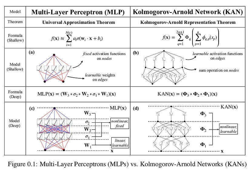
While MLPs have fixed activation functions on nodes (“neurons”), KANs have learnable activation functions on edges (“weights”). KANs have no linear weights at all — every weight parameter is replaced by a univariate function parametrized as a spline. We show that this seemingly simple change makes KANs outperform MLPs in terms of accuracy and interpretability. In summary, KANs are promising alternatives for MLPs, opening opportunities for further improving today’s deep learning models which rely heavily on MLPs.
According to the paper, much smaller KANs are comparable to or better than much larger MLPs in data fitting and PDE solving. Supposedly KANs possess faster neural scaling laws than MLPs. KANs can be intuitively visualized and can easily interact with human users, thus greatly enhancing interpretability.
This paper revolves aroundthe properties of the Kolmogorov-Arnold representation theorem for function approximation, which is the entire premise of every DL architecture.
- Representation Theorem Basics: Functions are decomposed into simpler functions that are then approximated using neural networks.
- Smoothness and Continuity: The goal is to ensure that the smoothness of the original multivariate functions is effectively translated into the neural network approximations.
- Space-Filling Curves: Function’s properties across dimensions, especially focusing on how continuity and other function properties are maintained or transformed in the approximation process.
What is a Spline and why does KAN need Spline?
A spline is a mathematical function used for creating smooth and flexible curves or surfaces through a set of control points. In mathematical terms, a spline is a piecewise polynomial function that maintains high levels of smoothness at the places where the polynomial pieces meet (the knots).

There are several types of splines, including:
- Linear splines: Connect the dots with straight lines, simple but not smooth. This is not differentiable at the dots.
- Quadratic and cubic splines: Second or third-degree polynomials to create curves. Cubic splines are widely used because they offer a good balance between flexibility and computational complexity.
- B-splines (Basis splines): Offer greater control over the shape of the curve, especially near the boundaries, and are defined over a set of control points that do not necessarily lie on the curve itself.
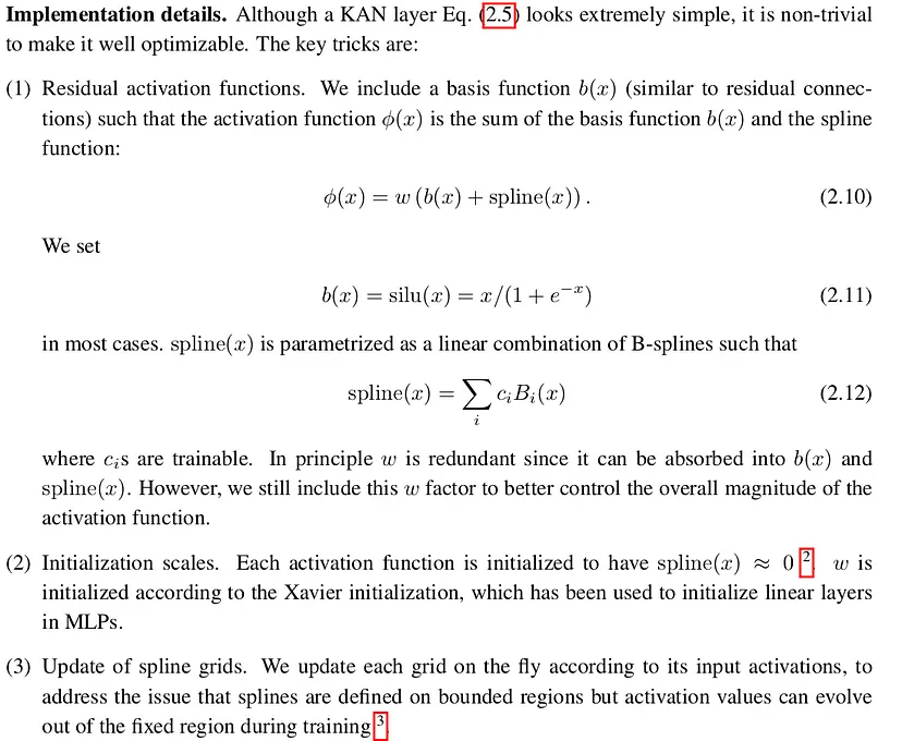
The paper uses B-Splines for KANs: Unlike basic splines, B-splines do not necessarily pass through their control points. Instead, these points guide the shape of the curve from a distance, providing a more flexible way of describing complex shapes and patterns.
B-splines are specifically useful in KANs due to their robustness in handling high-dimensional data and their ability to form smooth, multi-dimensional surfaces. For neural networks, where learning in high-dimensional data is standard, B-splines can be used to manage the complexity of the model without losing interpretability and while maintaining computational efficiency.
Kolmogorov-Arnold Representation Theorem
The core idea behind the Kolmogorov-Arnold Representation Theorem is that any (multi-variable) continuous function can be represented as a composition of continuous functions of one variable and the addition (+) operation. No matter how complex a multi-variable function might seem, it is possible to express it using simpler, univariate functions. It is similar to Fourier series which is a continuous, periodic function created by a summation of harmonically related sinusoidal functions.
Here’s the mathematical equation for Kolmogorov-Arnold Representation Theorem:
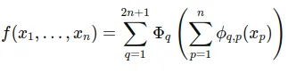
This theorem provides a way for deconstructing a complex multivariable function into a series of operations involving only one variable at a time, making it easier to understand and compute. This is particularly useful in contexts like neural networks, where such decompositions can help in designing architectures that efficiently approximate complex functions using simpler, easier-to-train components.
Understanding KAN
Traditional MLP Layers:
To understand let’s look at MLP as well. MLPs are based on the Universal Approximation Theorem, which states that a feedforward network with a single hidden layer containing a finite number of neurons can approximate continuous functions on compact subsets of 𝑅_𝑛, under mild assumptions on the activation function.:
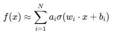
Here, 𝜎 is a fixed nonlinear activation function, 𝑤_𝑖 are the weights, 𝑏_𝑖 are the biases, and 𝑎_𝑖 are the output weights.
In typical MLPs, each layer consists of a linear transformation followed by a non-linear activation function. This means that for any given input, the network computes a weighted sum of the inputs and then applies a non-linear function like ReLU, sigmoid, etc., to this sum. MLPs are effective for many tasks but can be limited by the fixed nature of their transformations and the global effect of changes in parameters.
KAN Layers:
- Instead of the standard linear-plus-nonlinear approach, KAN layers use a matrix of 1D functions (e.g., B-splines) where each connection between two nodes in consecutive layers is defined by a separate function that can be individually adjusted.
- This structure provides a higher degree of flexibility and local control over the function approximation process. Each connection learns a specific part of the overall function mapping from inputs to outputs, potentially leading to a more nuanced understanding and representation of data.
But what is a KAN layer?
It turns out that a KAN layer with n_in -dimensional inputs and nout -dimensional outputs can be defined as a matrix of 1D functions.

A KAN layer is defined as a matrix Φ of 1D functions 𝜙_𝑝,𝑞 where 𝑝 indexes the input dimension and q indexes the output dimension. Each function 𝜙_𝑝,𝑞 has trainable parameters and maps an input directly to an output without the intermediary of a weighted sum followed by a universal activation.
Structure of KANs:
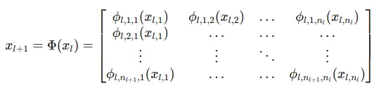
- Layer Definition: Unlike MLPs, each connection in a KAN layer is defined by an individual 1D function 𝜙_𝑙,𝑗,𝑖, which directly maps an input to an output (l is the l_th layer). This architecture does away with the matrix multiplication and instead uses a collection of function mappings where each function is responsible for transforming one component of the input to one component of the output.
- Function Matrix Φ: The entire layer can be described as a matrix of these functions Φ, where each function 𝜙_𝑙,𝑗,𝑖 is applied directly from each input node 𝑖 to each output node 𝑗. This setup provides a more flexible and tailored approach to data transformation:
The foundation of KANs is based on a supervised learning task where the goal is to approximate a function 𝑓 that maps input 𝑥_𝑖 to output 𝑦_𝑖 for all data points. The approach uses the Kolmogorov-Arnold theorem to decompose any multivariate function into a series of univariate functions and a sum operation:
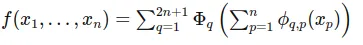
This equation implies that for each input dimension 𝑥_𝑝, there is a univariate function 𝜙_𝑞,𝑝, and Φ_𝑞 are higher-level functions that aggregate these univariate functions’ outputs.
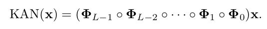
If we expand the above equation:
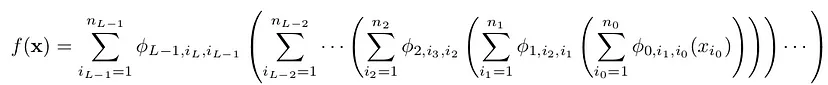
I know this is really complex, let’s write the simpler version of this and MLP so that it is easier to understand what’s happening in the end.

What does KAN offers?
- Flexibility: Due to the use of individual functions KANs offer greater flexibility at each connection, allowing each function to specifically adapt to features of the input data. On the other hand, MLPs use a more generalized approach with the same type of operation (linear followed by non-linear) applied uniformly across all inputs.
- Better Transformations: Each function in KAN can be optimized to perform a specific transformation, potentially making it better suited for heterogeneous data types or tasks where different input features require distinctly different processing methods.
- Interpretability: The use of individual functions in KANs might provide clearer insights into how each component of the input affects the output, as each function 𝜙_𝑙,𝑗,𝑖 could be analyzed independently.
- Computation: KANs might be more computationally intensive due to the diversity and number of functions being optimized, whereas MLPs benefit from the simplicity and efficiency of matrix operations. But KAN requires fewer parameters, thus making them faster.
Comparing KAN and MLP with an Example
To understand how these networks are different let’s take a simple example and compare the output of KAN and MLP.
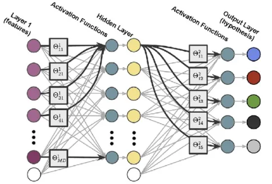
Multi-Layer Perceptron (MLP)
This is the basic structure of MLP:
Let’s assume the following configuration and values:
- Input Layer: 3 neurons
- Hidden Layer 1: 4 neurons
- Hidden Layer 2: 2 neurons
- Output Layer: 1 neuron
Weight Matrices:
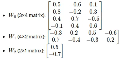
Input:

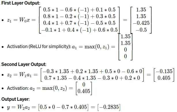
Computation for MLP:
Kolmogorov–Arnold Networks (KAN)
This is the basic structure of KAN:
Input:
Computation for KAN:
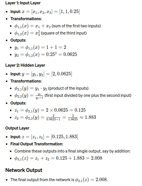
In the MLP, each layer performs a weighted sum followed by a non-linear activation function, while in the KAN, each “connection” applies a specific function (we are using random functions in our case) and aggregates these function outputs to feed forward.
Key Points
- MLP: Matrix multiplications are linear transformations adjusted by the weights. The non-linearity (ReLU in this example) allows the network to model non-linear phenomena.
- KAN: Each node connection applies a B-spline or another defined function, making it highly flexible and tailored to specific transformations needed per input feature.
Conclusion
KANs are shown to achieve comparable or even superior accuracy to MLPs while requiring significantly fewer parameters. KAN also offers enhanced interpretability due to their architecture, where each weight is replaced by a learnable univariate function parametrized as a spline. The paper highlights the mathematical elegance of KANs, grounded in the Kolmogorov-Arnold representation theorem, which provides a robust theoretical foundation for these networks. They require fewer training samples to achieve a certain accuracy level compared to MLPs.
This marks the end of this rather math heavy explanatory blog. The paper is really big and goes into much more detail, but beyond the scope of this blog.